Basic

• 為第四章基礎部份，紀錄符號的使用

kappa ϰ(G) - Separating set

唸做 kappa, 是為 connectivity，為 G 的最小 vertex 集合: S 的 size，其性質為 G-S 時會出現 disconnect 的現象，或是 G-S 只剩下 1 個 vertex（若 G 為 complete graph 時）

• 也就是 S 的 size 剛好是在構成 disconnect 要素的 threshold 上！

此時稱 graph G 為 k-connected，則表示其至少有值 = k 的 connectivity 存在！

• 而 S 則稱為 G 的 separating set，或是 vertex cut，S ⊆ V(G)，且 G-S 會有多個 component 產生(e.g. disconnect)

ϰ(G) 性質

• ϰ(Kn) = n-1 （Complete Graph）
• ϰ(G) <= n(G)-2 （當 G 不為 Complete Graph）
• ϰ(Km,n) = min{m,n} （當 G 為 complete bipartite graph 時，取較小的 partite size 為 ϰ ）
  • ϰ(K3,3) = 3 : 表示其 graph 可為 1-connected, 2-connected, 3-connected
• 當一個 graph 為 connected 且有 cut vertex，則其 > 2 個 vertices 時，connectivity > 1
• 若 graph > 1 vertex 時，其 connectivity 卻為 0 時，表示其 graph 本身便是 disconnected 狀態！
• ϰ(K1) = 0 （本身為一個 vertex 的情形，=0）

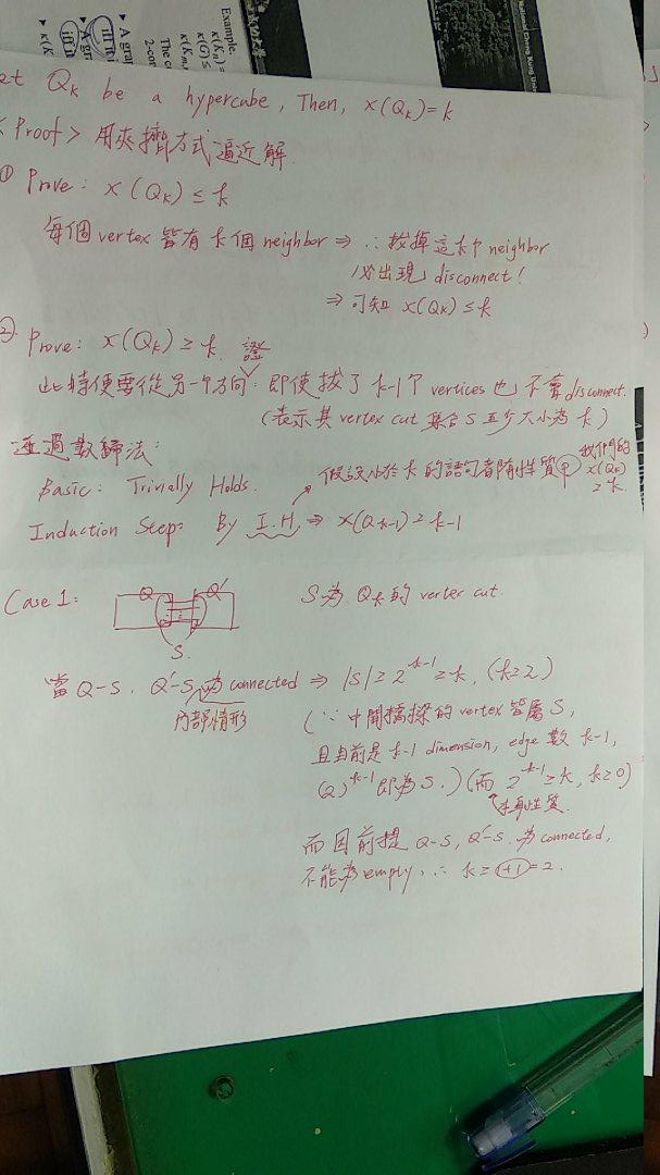
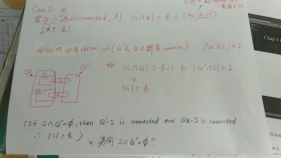
N 維度的 HyperCube

• 記做 Qn
• vertex 數量為 N=2^n
• 每個 vertex 上都以 n 個 bits 的二元字串來做表示 （也就解釋為何數量為 2^n）
• 每對鄰近的 vertices，兩兩之間只會有 1 bit 不同
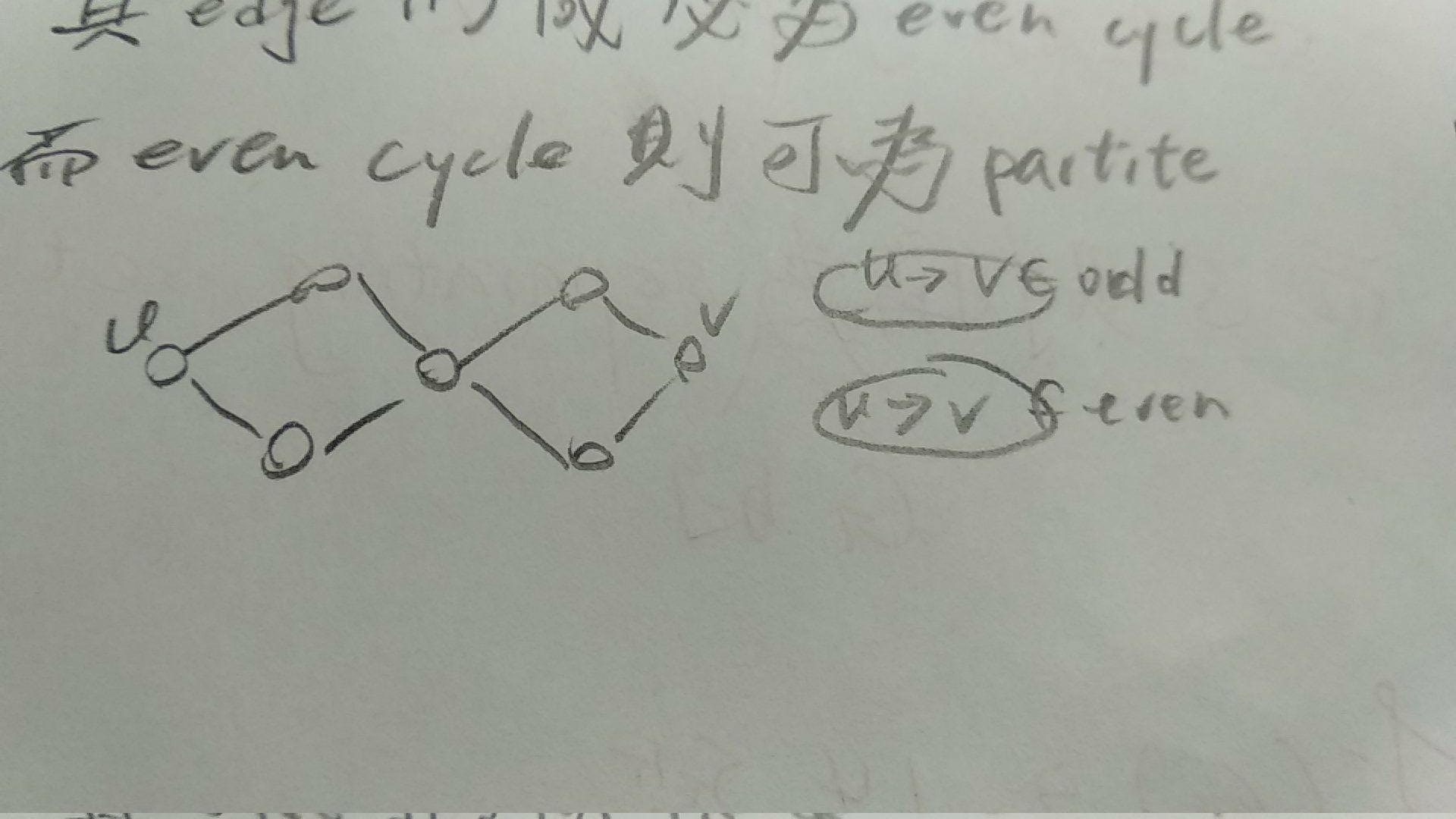
• Qn 為 bipartite graph

試證：
2 組 maximum matching 組合，其 edge 形成必為 even cycle
而 even cycle 則可以為 partite !

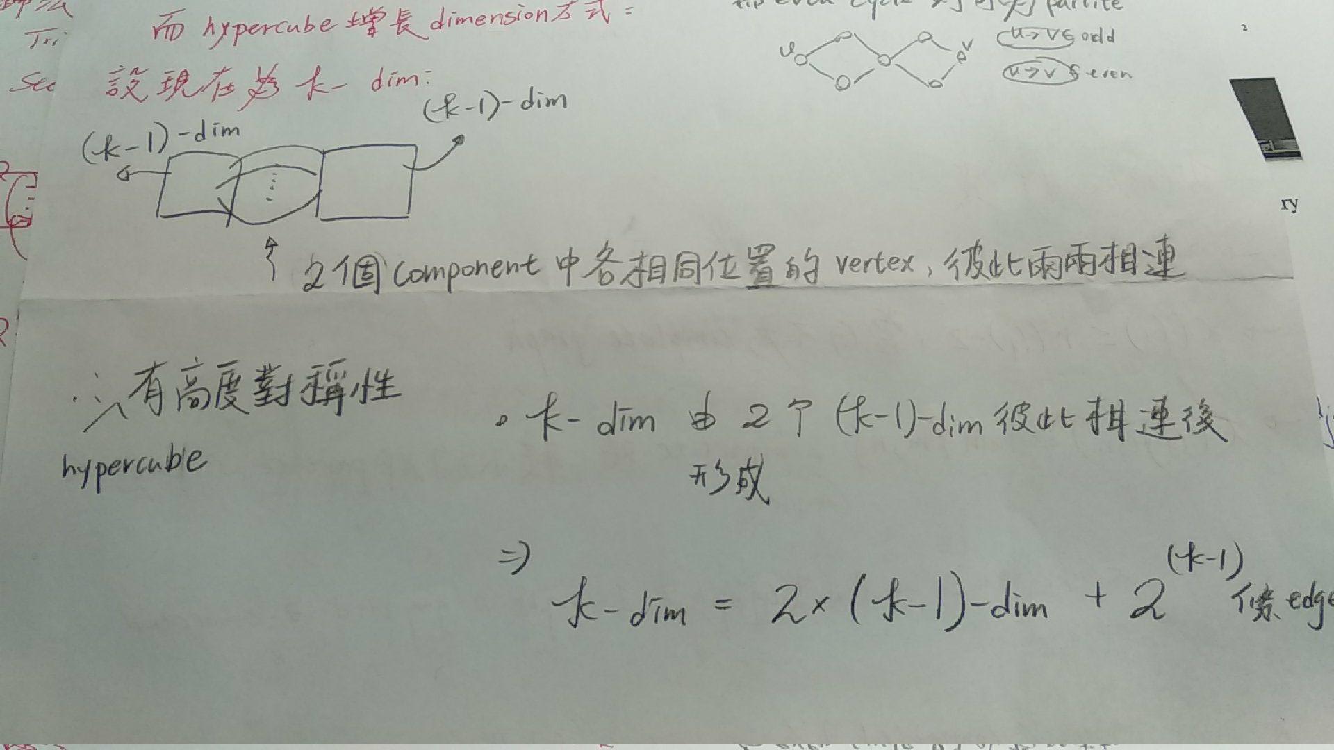
HyperCube 增長維度方式

ϰ'(G) - Disconnecting set

• disconnecting set:

  • 為 edge set（相比屬於 vertex 集合的 separating set）
  • 標為 F (⊆ E(G))
  • 使 G-F 有 > 1 以上的 component (使 G disconnect 的 edge set)

• 若一個 graph 其每個 disconnecting set 至少有 k 個 edges:

  • 則稱此 graph 為 k-edge-connected

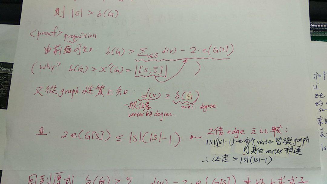
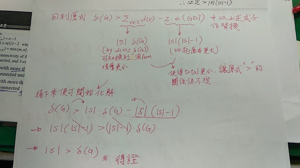
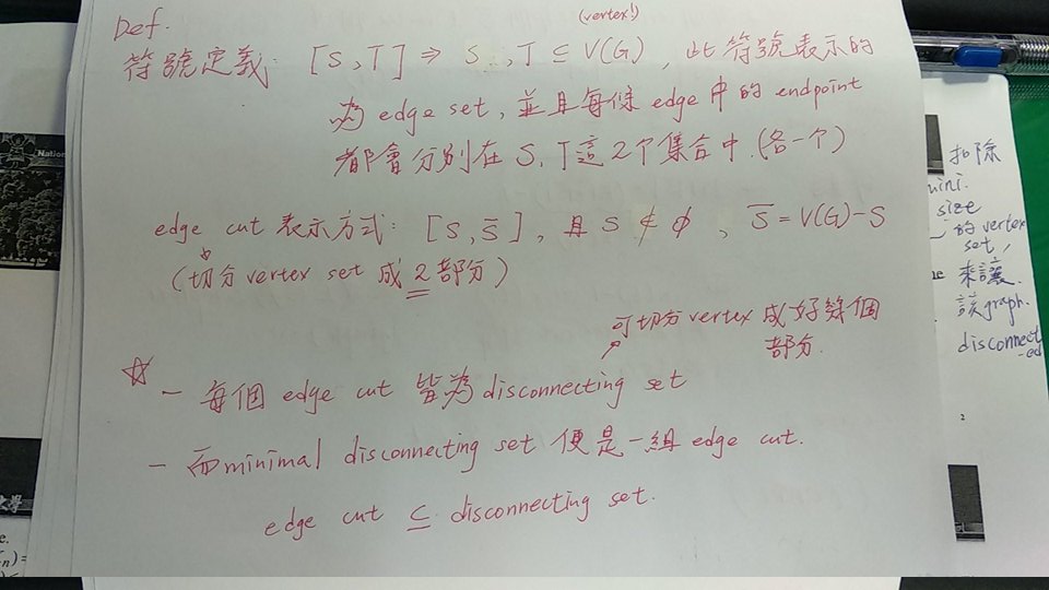
• edge-connectivity: ϰ'(G)，為 G 最小數量的 disconnecting set

Def - [S,T]

Def - line graph

• 標記為 L(G)，表示為 graph G 的 line graph
• 用以做 graph 的轉換（ 原本的 edge 會對應到 line graph 中的 vertex ）
• 所以在後面 (Theorem 4-2-19) 的時候，就會用到 Line Graph 的這項性質！
  • 並且在轉換時，會需要額外在端點加上偽 vertex，(讓原本端點 x,y 能夠搭配新加入的 vertex 形成 edge，並且轉換為 line graph 當中的 vertex )

Def - ear

• ear

  • 為 graph 中的 maximal path, 且其內部的 vertices 的 degree 皆為 2 (不包括端點)

• ear decomposition

  • 為 graph 中由一個 cycle P0 開始，依序加入 P1, P2, ..., Pk，當後續加入的 Pi (當 i > 1) 對目前 graph 而言為 ear，則稱為 ear decomposition（e.g. if k=2, 若 P2 為 ear 的話，則 P0 ∪ P1 ∪ P2 稱為 ear decompostion ）

• closed ear

  • 為一 cycle C 於 graph G 當中，並且這個 C 上除了一個跟 G 相接的 vertex (i.e. 這個 cycle 的起點與終點也是這個 vertex!)之外，其餘 vertex 的 degree 皆為 2

• closed-ear decomposition

  • 和 ear decomposition 相同，只不過在這邊 Pi(i > 1) 可以是為 open ear 或是 closed ear

• ear/closed-ear 皆有 theorem，參考 ear theorem 頁籤

Prove ϰ(G) of hypercube

• Figure 1

• Figure 2

探討 Case 2

• 理解： 由於 Q 為 hypercube 型式，切分兩個 component 的 S 與 其中一側做聯集 的大小至少為 k-1 （在 case 中由於以數歸法，所以探討為 k-1 維度）
• 而 case 2 情況為扣除 S 之後，有一側會出現兩個 component；則可以知道，該側與 S 的聯集必定大於 k-1，形成 聯集結果 >= k 的結果
• 總和必要性與充份性，證實 k 維度的 hypercube 的 ϰ 等於 k

Harary Graph

Type

• 性質 + Type 1

• Type 2

• Type 3

Theorem - Harary Graph 的 edge 數量

Theorem

• 在 simple graph 中，探討 ϰ(G), ϰ'(G), mini-degree 之間的關係

Theorem: 3 regular graph

• 探討在 3-regular graph 情形下的狀況， ϰ(G) = ϰ'(G)

Proof

Proposition

• 探討 S 與 S的補集 間所有的 edges 數量

Corollary

• 若 G 為 simple graph 且 |[S,S補集]| < G 的 mini-degree, S 不為空集合且屬於 G vertex set，則 |S| > G 的 mini-degree

• Proof

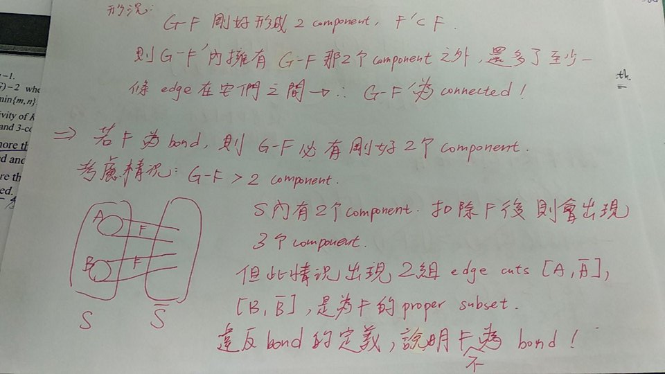
Def - bond 的定義

bond 為一最小的 non-empty edge cut (e.g. => 為 cut-set, 並且其內部 沒有任何其他的 proper subset 的 cut-set 存在)

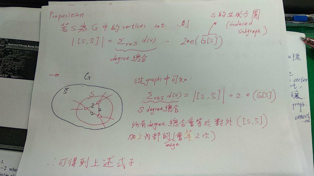
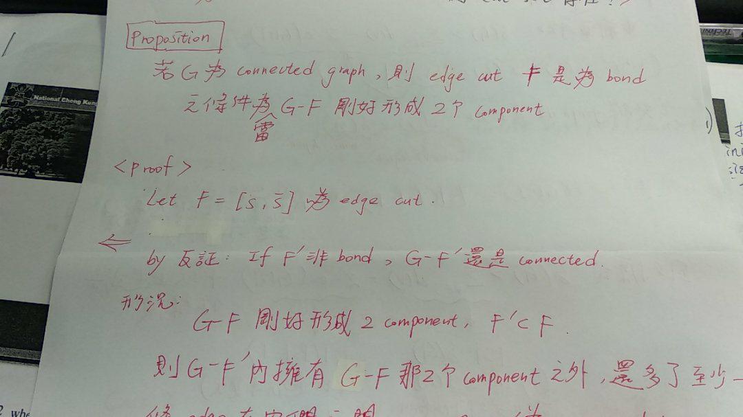
Proposition

k-connected

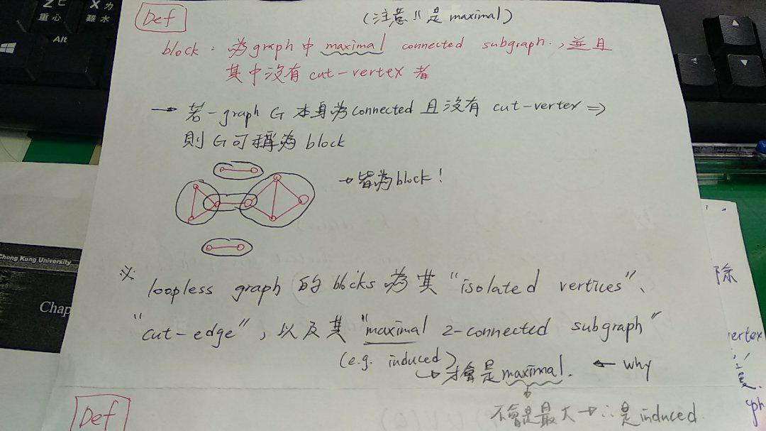
Def - block

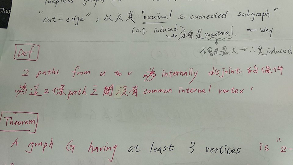
Def - internally-disjoint

Theorem - 4.2.2

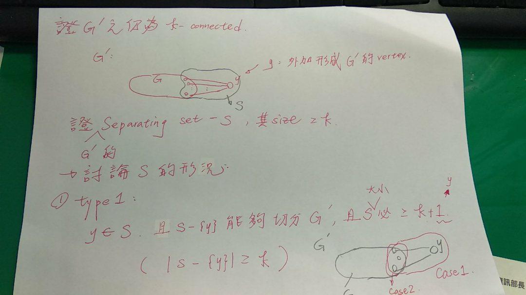
Lemma

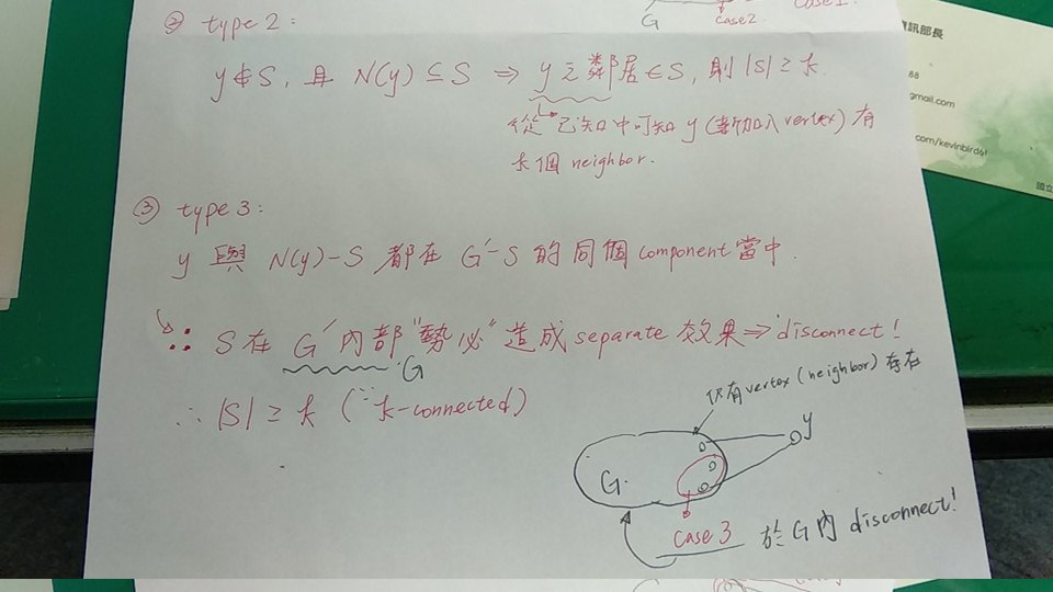
當 G 為 k-connected graph，且 G' 是從 G 加上一個新的 vertex: y（並讓 y 擁有 k 個於 G 中的 vertex 做鄰居），則 G' 仍為 k-connected

• Proof

Theorem - equivalent 情況

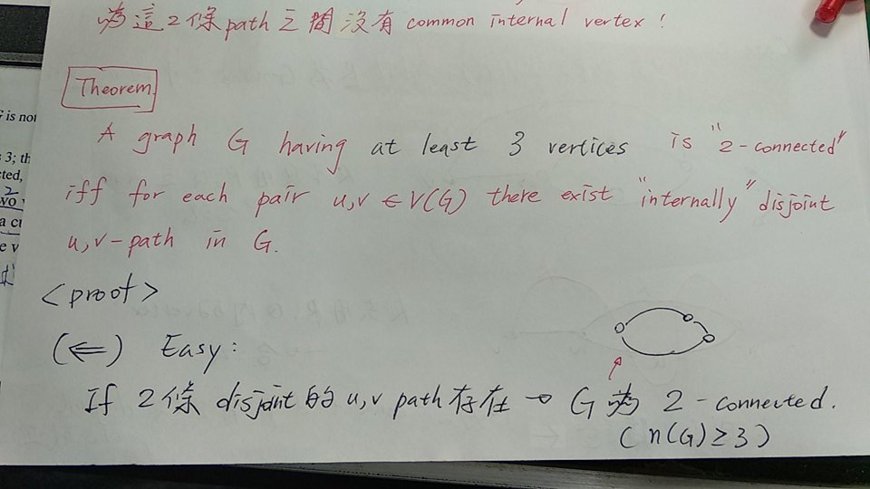
對於一個擁有至少3個 vertices 以上的 graph G 來說，以下情況為等價：

A) G 為 connected 且沒有 cut-vertex

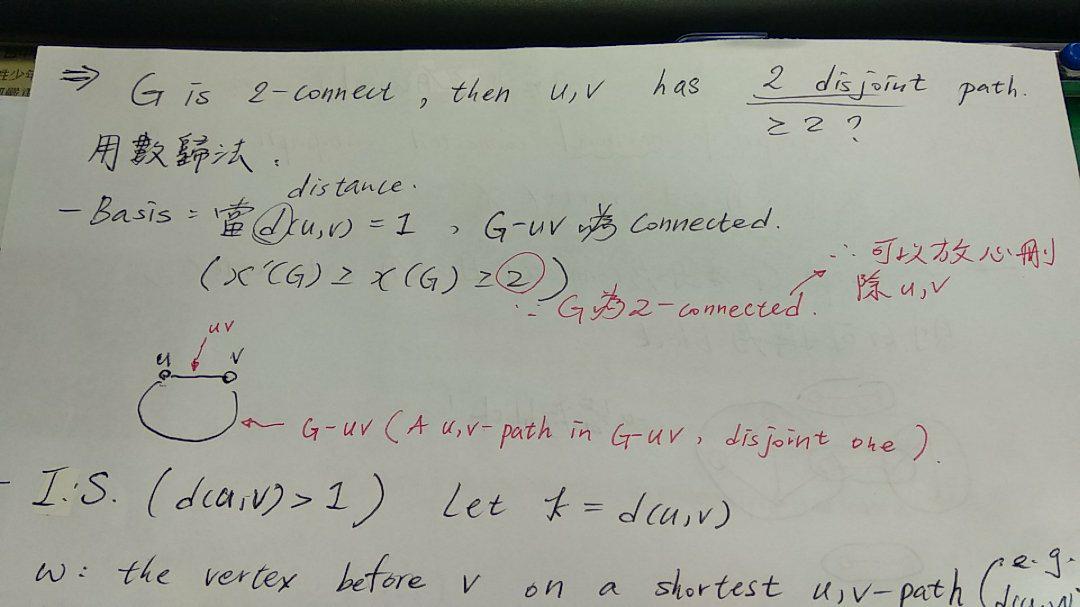
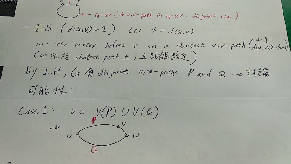
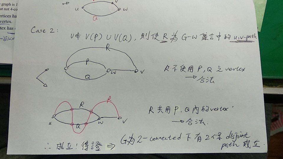
B) 對於屬於 G 的 vertex x,y,， 內部存在不相交的 x,y-paths

C) 對於屬於 G 的 vertex x,y,, 存在一個 cycle 穿過 x,y

D) δ(G) >= 1，且所有 pair of edges 會剛好在同一個 cycle 上 （e.g. 一定存在一 cycle 經過這 2 條配對邊）

Prove - A) <=> B)

由 Theorem 4.2.2 （上面）來做證明！ 說明 A 與 B 互為等價

Prove - B) <=> C)

透過兩條 disjoint 的 x,y-paths 來組合這個通過的 cycle

Prove - D) => C)

• 從 δ(G) >= 1 可以知道， x 和 y 不是孤立點
• 再透過 D 內性質： pair of edges 落在同一個 cycle 上來說明，存在一 cycle 穿過 x,y

Prove - A) ^ C) => D)

• G 若為 connected，則表示 δ(G) >= 1 （D 的性質）
• 再來考慮兩條 edges: uv, xy
• 透過 subdivision 的方式從中生出一個中間點 w,z ；透過新生成的這兩條 edge: uwv, xzy 來構成 cycle （ by 性質 C）
• 接著再刪除 subdivision 產生的新 vertex，來還原成原本的 edges；而這時可以知道，仍為兩條 disjoint edge； 那麼就可以證實， 原先這兩條 uv, xy 在這個 cycle 上（只是透過原先 uv, xy 來取代生成 cycle 的 uwv, xzy）
• 這樣就可以完成由 A 和 C 的聯集等價於 D 的結論

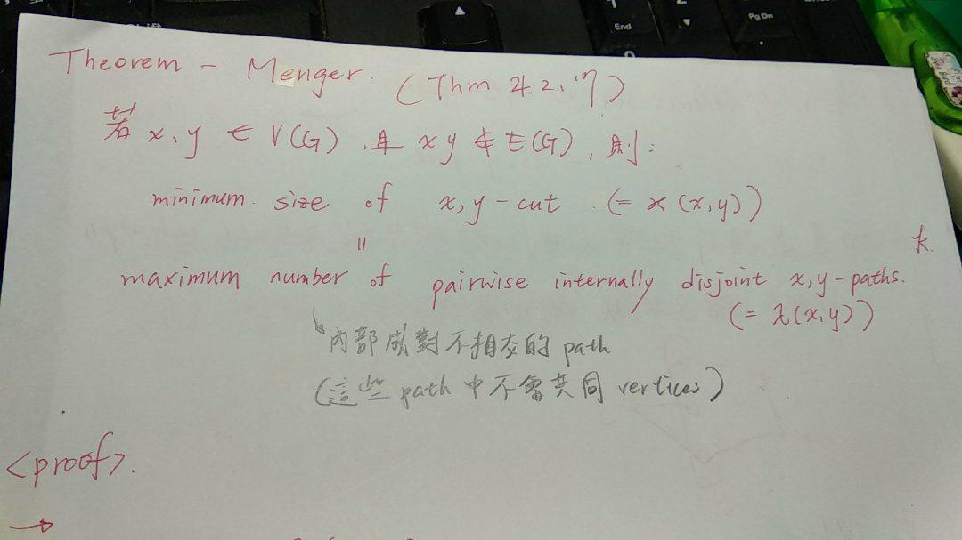
Theorem 4.2.17 - Menger Theorem

性質

• 兩點之間的 vertex cut 的最小值: ϰ(x,y)，會等於其內部 pairwise disjoint x,y path（內部成對、不相交，不使用共同 vertex的 paths ） 的數量最大值: λ(x,y)

• 主要概念： 若存在兩點 x,y 並且他們之間不存在互相連通的 edge 時，這個時候我們便可以套用 Menger 定理！

  • 透過兩點之間的 pairwise disjoint path、以及 vertex cut 間的關係來說明幾項特性！
  • 像是 subdivision、line graph 等動作，都是為了要達到 Menger Theorem 所需要的狀態： 兩個不相鄰的 vertices，所加入的額外操作！

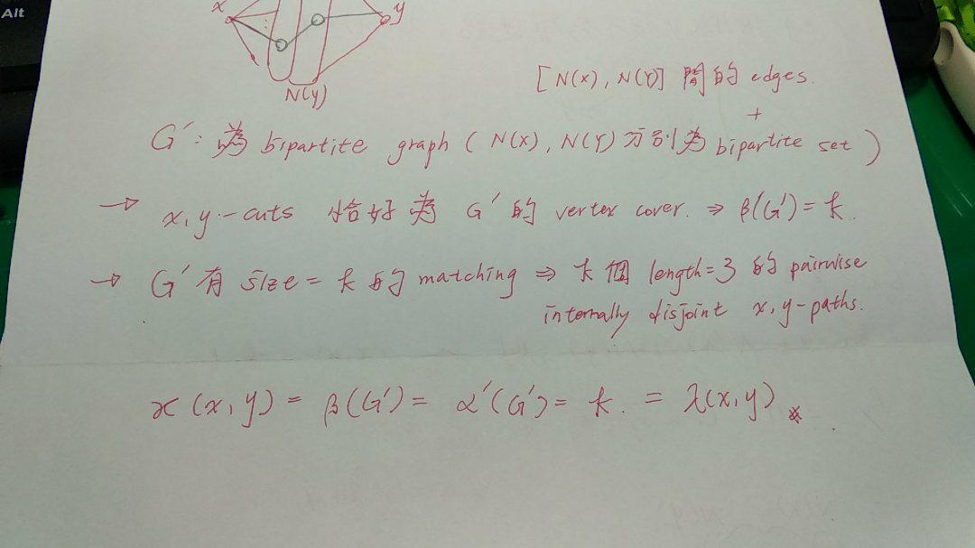
=> ϰ(x,y) = λ(x,y) by Menger 定理

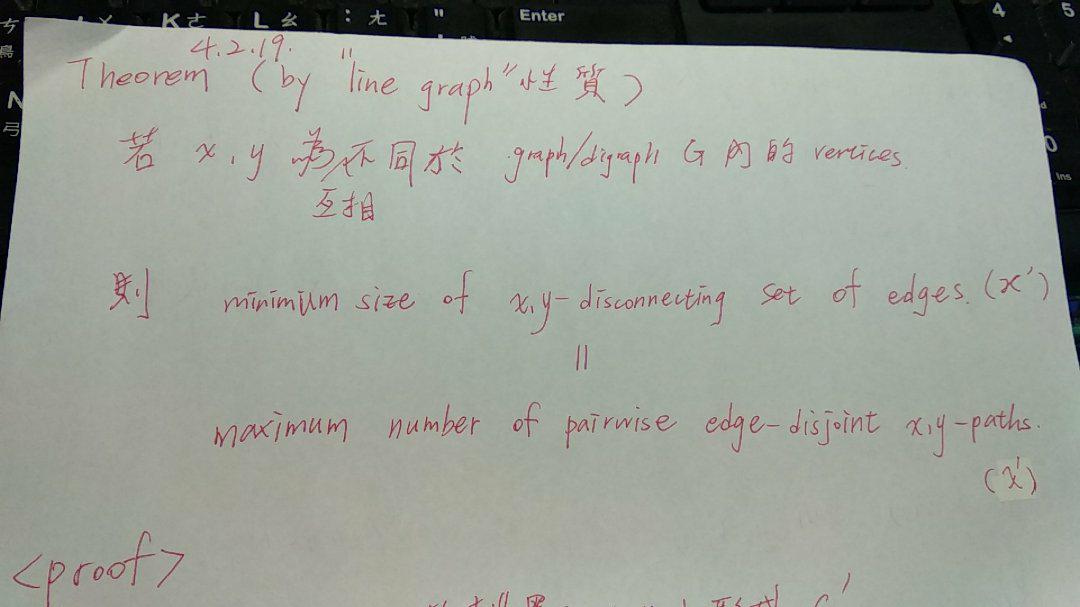
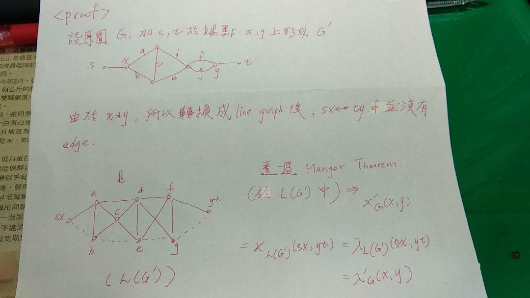
=> ϰ'(x,y) = λ'(x,y) by Menger 定理(Edge 版本)， Theorem 4.2.19 （這個就透過 line graph 來從 edge 轉換成 vertex 後套用 Menger 定理來證明！ ）

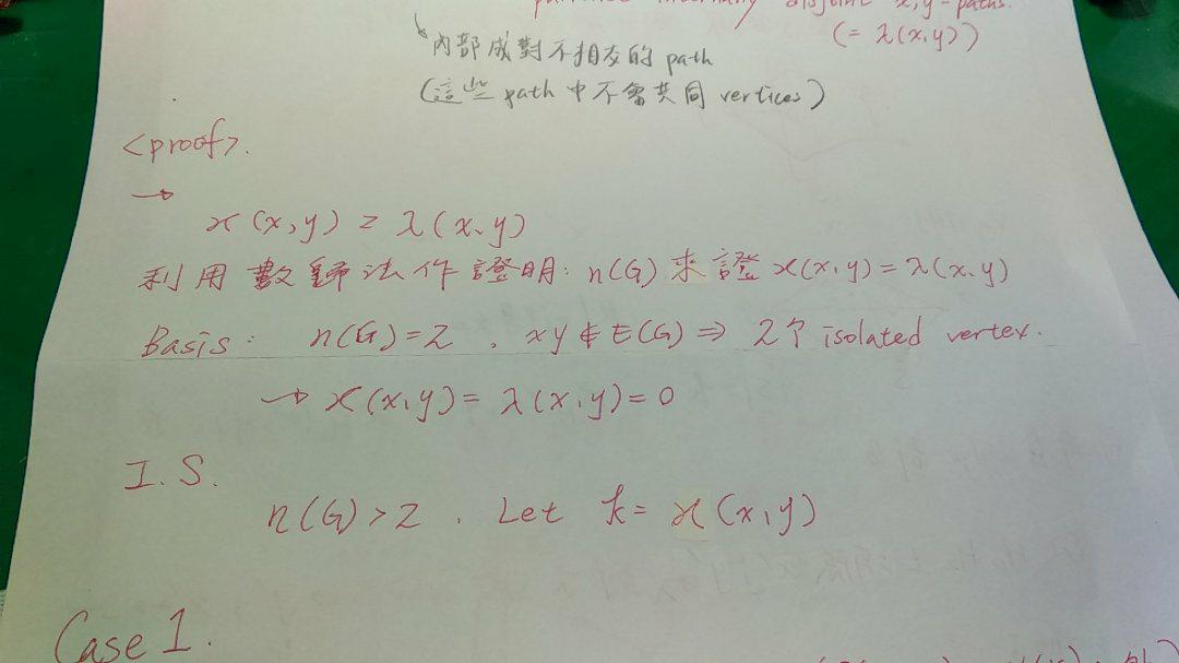
Proof

• 證明主要透過節點數量 n(G)的狀況來做分析，並透過數學歸納法做證明

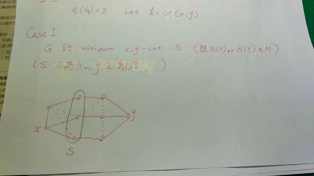
Case 1

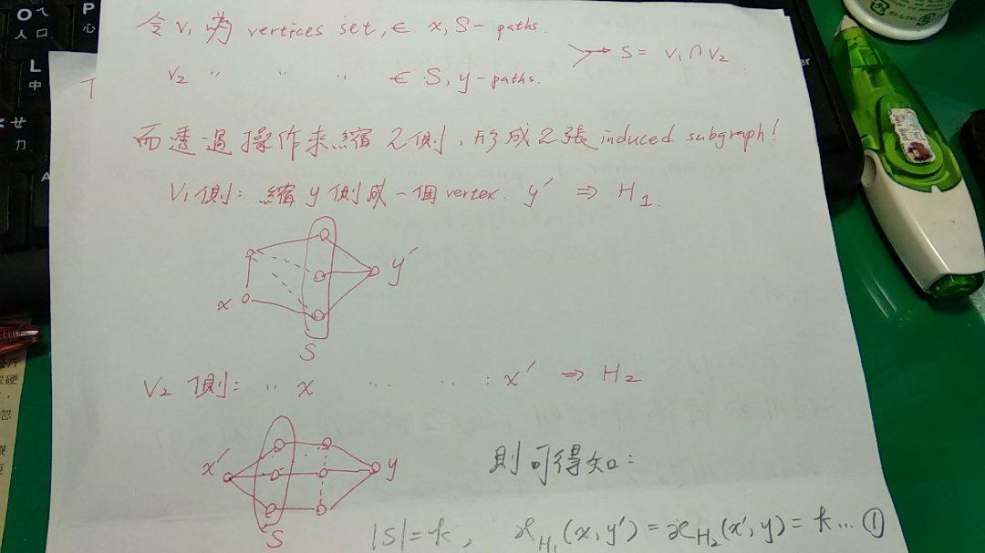
Case 1 狀況為: 假設 x,y-cut: S 集合不為 x,y 的鄰居時的情況做分析

Case 1-1

藉由使得 x 側、 y 側收斂來說明，|S| = k， ϰ(x',y) = ϰ(x,y') = k (Case 1 中 connectivity 的部份)

Case 1-2

從收斂的兩張圖可以看出，λ(x',y) = λ(x,y')，進而可以刪除 x',y' 來還原成原圖，可得 λ(x',y) = λ(x,y'), λ(x',y) = λ(x,y') = λ(x,y) = k( Case 1 中 pairwise disjoint x,y path 的部份)

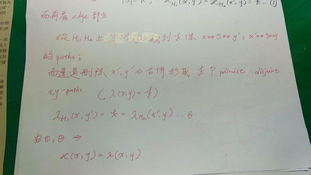
結合 Case 1-1 以及 Case 1-2，可以知道在 Case 1 假設情況下， ϰ(x,y) = λ(x,y)；接下來準備進入另一個狀況討論：

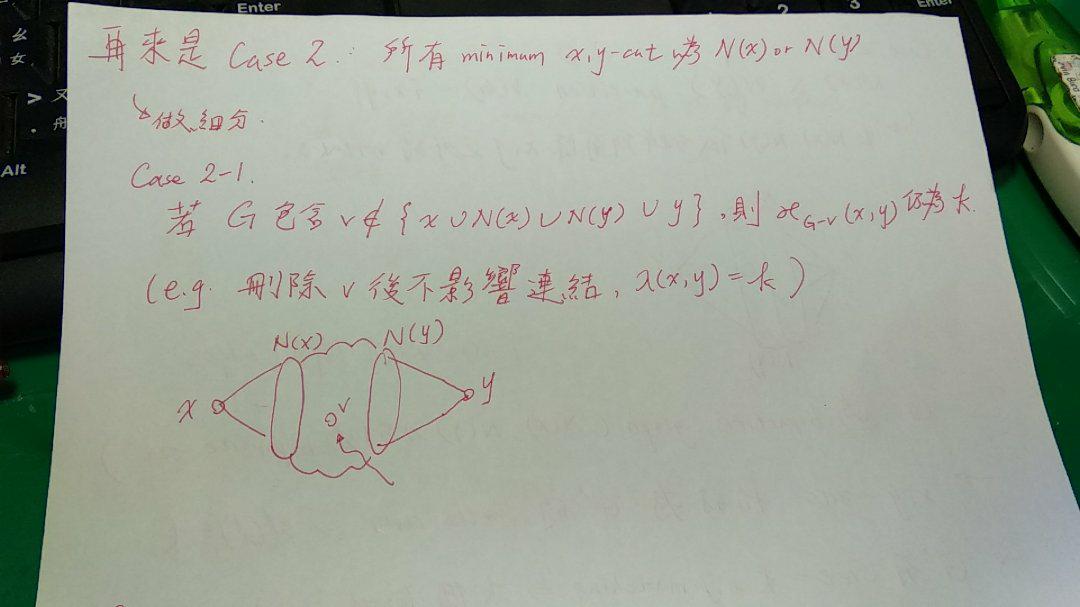
Case 2 + Case 2-1

當 x,y-cut: S 集合為 x,y 的鄰居時的情況：

Case 2-1: 情況為 "當 N(x), N(y) 之間還有存在其他 vertices 時"

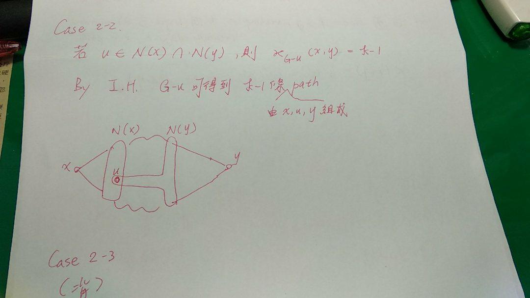
Case 2-2

Case 2-2: 情況為 "當 N(x), N(y) 之中，有部份 overlap 情況發生時"

Case 2-3

Case 2-3: 情況為 "當 N(x), N(y) 互為 bipartite 之中的 partite set 時"

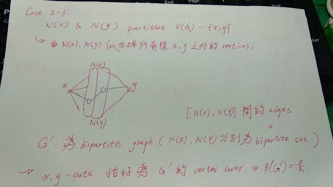
Summary

Case 2 則同樣透過這三種情況來說明 "ϰ(x,y) = λ(x,y)"

Theorem 4.2.19

• 透過 line graph 性質來證明
• 等同於 Menger Theorem 的 edge 版本

Proof

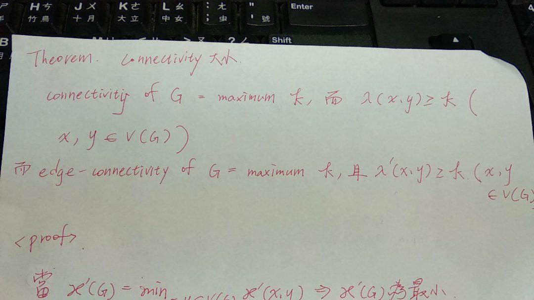
Theorem

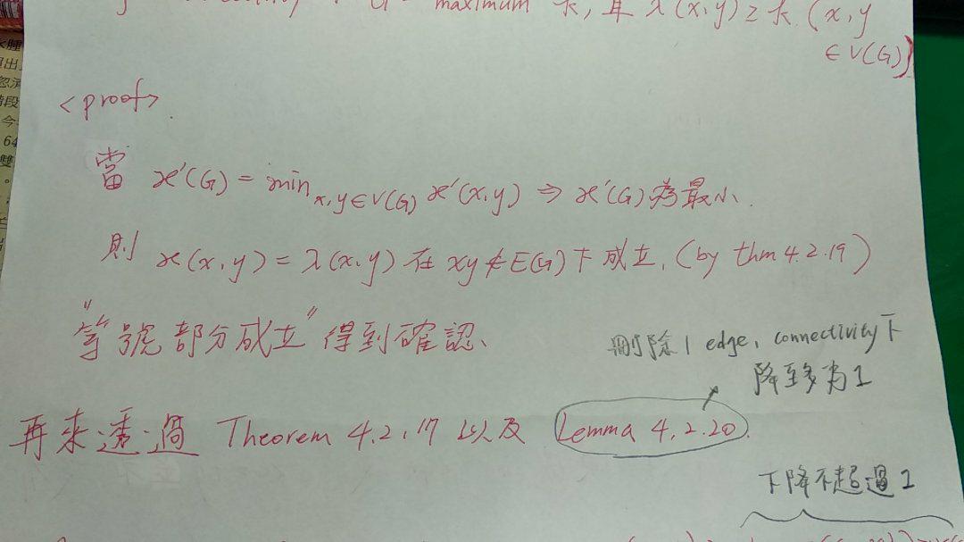
計算 connectivity 以及 edge-connectivity ，以及 disjoint x,y-paths、 edge-disjoint x,y-paths 這兩對配對間大小

其中 λ(x,y) 為表示從 x 到 y 之間 pairwise 的 internally disjoint x,y-path 的數量 （ λ'(x,y) 則為 edge-disjoint x,y-paths set ）

這邊主要講述跟 ear 相關的幾個定理說明，包括 ear/closed-ear、strong orientation

Theorem - ear

當一個 graph G 是為 2-connected 時，表示 G 有一個 ear decomposition; 並且每個 cycle 於 2-connected 的 graph 中皆為某個 ear decomposition 的 initial cycle

• Proof:
  • 先從 Sufficiency 證明起 （若 G 有 ear decomposition，則 graph 為 2-connected）
  • 假設現在 graph G 為 2-connected, 則 G 滿足條件：能夠再加入任何一個 ear 後保持 2-connected 的狀態 ->
    • 設現有的 graph G 狀態為 2-connected (i.e. 擁有 ear decomposition)
    • 則此時從上面找到兩點： u,v ，並且構成一個新的 ear : P (uv 間做 subdivision 的動作後，使得符合 ear 的定義："所有內部存在的 vertices ，其 degree 皆為 2" 的條件)
      • subdivision 會保持 2-connected!
    • G + uv 仍為 2-connected（於此適用於繼續以相同方式加入 ear! graph G 仍會保持 2-connected）
  • 再來是 Necessity 的部份 （若 G 有 2-connected，則表示 G 有 ear decomposition）
  • 假設目前存在一個 graph G，其為 2-connected； 且存在一個 Cycle C 於 G 當中
  • 則此時從這個 cycle C 作為 ear decomposition 的 initial cycle 開始，逐一加入 ear 進去；做一個 iterative 的動作；
    • iterative 動作：
    • 挑選非目前 ear decomposition 的兩個 vertices（u,v），再從 ear decomposition 上挑選兩個 vertices（x,y）
    • 使這 4點 構成一個 cycle，這麼一來就形成新的 ear decomposition 了！
  • 停止條件為，當目前的 ear decomposition 等於當初的 graph G 時，就停止
    • 所以當 iterative process 結束時，便可得到一個擁有 2-connected 性質的 ear decomposition - G

Theorem - closed-ear

當一個 graph G 是為 2-edge-connected 時，表示 G 有一個 closed-ear decomposition; 並且每個 cycle 於 2-edge-connected 的 graph 中皆為某個 decomposition 的 initial cycle

（跟上面的定理類似，只是從原本針對 vertex 的 2-connected 換成 2-edge-connected）

Theorem - strong orientation

當 graph G 存在強方向性（該 graph 中所有的 undirected edge 全部替換成 directed 時稱之），則表示 G 為 2-edge-connected!

• Proof
  • Necessity：
    • 當 graph G 存在 strong orientation 時，表示 G 不可能為 disconnected、並且不存在 cut-edge! ( strongly orientation 的性質其中就有 bridgeless，所以不會存在兩個 component 之間只有單向的 directed edge 存在的情形 )
  • Sufficiency:
    • 當 graph G 有 2-edge-connected 性質存在時，則其有一個 closed-ear-decomposition =>
    • 跟前面 ear 的定理證明類似，從 initial cycle 出發，把 initial cycle 上所有的 edge 做 orient，形成必要條件: strongly orientation
    • 接著再一一加入新的 ear（跟前面的加入方式相同），並把這些新 ear 上面 edges 做 orient
    • 藉此可以得證！

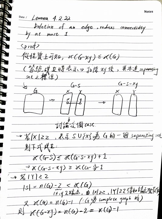
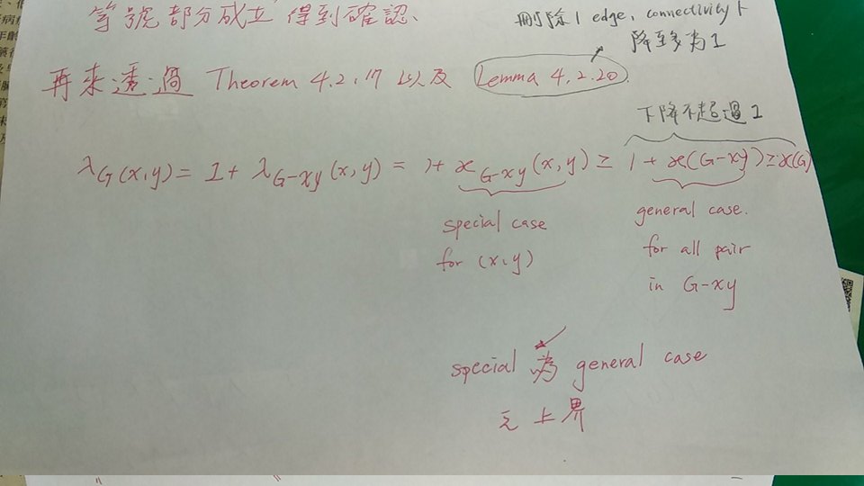
Lemma 4.2.22

主要證實性質： graph 在扣除一條 edge 後，最多減少 1 個 connectivity !

=> ϰ(G - xy) <= ϰ(G)，透過指出兩種情況： ϰ(G - xy) = ϰ(G) 以及 ϰ(G - xy) = ϰ(G) - 1 來做說明

Network Flow

• 每條 edge 上都會有一個實際的 flow 值（f(e)），以及 capacity 的值（cap(e) or c(e)）

• 起始點： source vertex (s)； 終點： sink vertex (t)

  • 每個 vertex 可稱為 node
  • 而每個 node v 都會有流進與流出，分別標示為 f-(v) 以及 f+(v) （注意： 流進是帶負號的！）

• 並且有兩種方向：

  • 從 source 到 sink 的稱之為 forward path； 而反過來的則稱為 backward path

• 當一個 flow 為 feasible 時，表示其滿足：

  • 0 <= f(e) <= c(e)
  • 且除了 s,t 之外的 node，都滿足 流進 = 流出

• 而由於除了 s,t 之外的節點都是持平，所以我們計算一個 flow：f 值（ 標記為 val(f) ）的時候，針對 sink vertex 做運算即可： f-(t) - f+(t)

  • 並且在 val(f) 達最大值時，表示此 flow 為 feasible flow 中的 maximum flow

• f-augmenting path & tolerance: z:

  • 表示現階段的這條 flow 不是最佳解，還能夠增加 cap !
  • 接下來我們來看 f-augmenting path 的定義；需要滿足以下條件，才可稱為 f-augmenting path：
    • 若此時為 forward direction: 則 f(e) < c(e)
    • 若此時為 backward direction: 則 f(e) > 0
  • 滿足以上條件，並且能夠從 source vertex 到 sink vertex 皆滿足，則此條路徑可稱為 f-augmenting path!
  • 如此我們可以計算其中的 tolerance: z:
    • tolerance 計算方式：
      • forward: z = c(e) - f(e)
      • backward: z = f(e)
    • 然後取得 path 上 z 的最小值，便是 tolerance
  • 而有了 tolerance 後，我們可以重新計算、改變這條 f-augmenting path( f )成為更加 feasible 的解 ( f' ) :
    • forward 的 edge 皆 +z； backward 的 edge 則 -z；
    • 所以新的 val: val(f') = val(f) + z
    • 會比舊有的值多出 z！

• source/sink cut [S,T]

  • 為切分 source, sink 的 edge cut
  • 只包含 forward 的 edge ！
  • 並且當 flow: f 為 feasible 時，會符合：
    • val(f) <= cap(S,T)

• Max-flow Min-cut Theorem （Ford and Fulkerson）:

  • 這個定理是上面尋找 f-augmenting path 並轉換為 more feasible 解的演算法
  • 主要從輸入的 graph （network flow）中找到 f-augmenting path 後，透過運算獲得 tolerance 後更新這條 f-augmenting path
  • 直到沒有 f-augmenting path 存在後，即可從現有的 source-sink path 當中，找到最大值的 val，即可宣稱其為 network 中***最大的 feasible flow 值***，或是 最小的 source/sink cut 的 capacity
  • val(f) = f+(S) - f-(S) = f+(S) = cap(S,T)